ANN at Scale: HNSW

Exact k-nearest-neighbor compares the query to every vector: correct, and hopeless at a billion of them. The escape is to stop demanding the exact answer. Accept a rare near-miss and you can search that billion in a few milliseconds. This is the data structure that makes the trade.

Suppose you want the nearest coffee shop and you find it by walking to every coffee shop in the city and measuring each one. Correct, and absurd. In reality you take the main roads toward the right neighborhood, then check the few places on that block. Approximate nearest neighbor search does the same across a map of a billion points: follow the highways, skip almost everything, and accept that once in a while you end up a block off.

The trade: approximate

Exact search guarantees the true k nearest, and pays for it with N comparisons per query. Approximate nearest neighbor (ANN) drops the guarantee. It returns the true nearest most of the time and a very close neighbor the rest of the time, while touching only a tiny fraction of the vectors.

The quality of an ANN index is measured by recall: of the true top k, how many did it actually return (recall@10 = the fraction of the real top ten it found). In practice you can tune an index to 95 to 99 percent recall while visiting a small sliver of the data. For search and RAG, the occasional near-miss barely matters, and the speedup is the difference between milliseconds and minutes. That trade is why every production vector database is approximate.

Navigable small worlds

The dominant ANN method is HNSW, Hierarchical Navigable Small World graphs (Malkov and Yashunin, 2016). Start with the small-world part.

Connect every vector to its M nearest neighbors, forming a graph. To search, begin at some fixed entry node and hop greedily: look at the current node's neighbors, move to whichever is closest to the query, and repeat until no neighbor is closer than where you already are. Because the graph is a "small world", any two nodes are only a few hops apart, so you arrive in the query's neighborhood after visiting a handful of nodes rather than all of them.

Here is exactly that greedy walk. Drag the query, then step or run the search from the entry node. The dashed ring is the true nearest, so you can watch greedy either land on it or settle for a near-miss:

Notice two things. It visits only a few of the 34 nodes, which is the whole point. And it can converge on a node that is close but not the true nearest, which is the approximation you are trading for that speed.

The hierarchy (the H in HNSW)

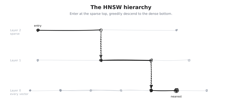
A single greedy layer can wander or get stuck. HNSW fixes this with layers, borrowing the idea of a skip list. The top layer holds a few nodes joined by long-range links; each layer down has more nodes and shorter links; the bottom layer contains everyone.

Search starts at the top, greedily gets roughly close using the long hops, drops down a layer, refines with shorter hops, and repeats down to the bottom layer where the final answer lives. The sparse top covers distance fast; the dense bottom pins down the exact neighborhood. The result is search that scales roughly logarithmically with the number of vectors instead of linearly.

The knobs

Three parameters trade recall against speed and memory:

• M is the number of neighbors each node keeps. A higher M means a denser, better-connected graph and higher recall, at the cost of more memory.
• efConstruction is how hard the algorithm searches while building the graph. Higher means a better graph and higher recall, at the cost of slower indexing.
• ef (efSearch) is the size of the candidate list kept during a query, effectively a beam width. ef = 1 is the pure greedy walk the explorer above shows; a larger ef explores several paths at once and rarely misses, at the cost of visiting more nodes. This is the main dial you turn at query time to buy recall with latency.

The same database, two ways

Enough abstract dots. Here is a real query against a small food database, answered both ways on the same data. Run it in Scan (kNN) and it checks every item; switch to Graph (HNSW) and it hops through just a handful of them to the same answer. That gap, every item versus a few hops, is the entire reason ANN exists, and on a real index it is a billion comparisons versus a few dozen hops.

In production

HNSW is the default approximate index almost everywhere: OpenSearch and Elasticsearch k-NN, FAISS, pgvector, Weaviate, Qdrant, and Milvus all build one. When you switch on vector search, you are almost certainly switching on an HNSW graph underneath. It is the reason a billion-vector index can answer in single-digit milliseconds at high recall, which is the entire reason semantic search is practical at scale.

We now have two strong but different tools: lexical search (BM25) that nails exact terms, and vector search that matches meaning. Each is weak exactly where the other is strong. The next part puts them together: hybrid search.