How RAG Finds Things

Finding the right page is the hard part of an open-book exam. Turn to the wrong one and even a brilliant student writes a wrong answer, so most of the grade rides on how you locate the passage, not on how you write. This piece is about how RAG turns the pages: the different ways it decides which passages count as relevant to a query.

This is part of a series on RAG. The opening piece argued that RAG quality is mostly retrieval quality. So start where it matters most: how a RAG system decides that a chunk matches a query. There are more options here than people realize, and the good systems use several at once. We will take them one at a time, each with an everyday analogy first, then the real mechanism, then a demo.

Sparse: match the exact words

Think of the index at the back of a book. It lists exact words and the pages they sit on. Look up "car" and you jump straight to every page with that word. But if the author wrote "automobile" throughout and you look up "car," the index is silent, even though the whole book is about cars. It matches letters, not meaning.

That is sparse retrieval, and BM25 is the classic recipe for it (a tune-up of the older TF-IDF). It scores a document by the query words it actually contains. But not every match counts the same, and that is the clever part. BM25 weighs three simple things, and the visualizer below lets you turn each one and watch the score move.

• How often the word appears (term frequency). A page that says "defibrillator" five times is more about defibrillators than one that says it once. But the bonus fades fast: after a few mentions, each extra one barely helps. Saying a word fifty times does not make a page fifty times more relevant. The dial called k1 sets how quickly that bonus levels off.
• How rare the word is (term rarity). Common words tell you nothing. "The" is on every page, so it is no help in finding anything. "Defibrillator" is rare, so on its own it almost points at the right page. Rare words count for far more than common ones.
• How long the document is. Finding "defibrillator" in a one-line note is a stronger signal than finding it buried in a 500-page manual that was always going to contain lots of words. So BM25 quietly discounts long documents, so they do not win just for being long. The dial called b sets how hard that length counts against a document.

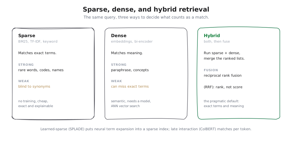
Why go to all this trouble? Because sparse retrieval has real strengths. It needs no training, it is cheap, and it is exact. Product codes, error messages, function names, people's names, legal citations: these are where meaning-based search quietly fails and plain word-matching quietly wins. Its weakness is the mirror image: it is blind to meaning. Ask about "cars" and a document that only ever says "automobiles" is invisible, because the two share no word. That gap is called the vocabulary-mismatch problem, and it is exactly what dense retrieval was built to fix.

Dense: match the meaning

Now imagine a librarian who has read everything and understands what you mean. Ask for books about "cars" and she also hands you ones about "automobiles," "vehicles," even "sedans," because she matches the idea, not the spelling. That is the leap from letters to meaning.

Dense retrieval embeds the query and each chunk into a fixed-length vector with a neural model called a bi-encoder. Picture two people who each jot a one-line gist of their own text without ever seeing the other's, and then you compare the gists: a bi-encoder is that, encoding the query and the chunk separately so that semantically similar texts land near each other. "Cars" and "automobiles" end up close, and retrieval becomes a nearest-neighbour search in that space. Comparing the query against every chunk exactly would be too slow at scale, so it is made fast by approximate nearest-neighbour (ANN) indexes: instead of checking every book in the library, you walk straight to roughly the right shelf and look only there, giving up a tiny chance of missing the single best match for an enormous speed gain. The foundational version of this for RAG was DPR, dense passage retrieval.

Its strength is paraphrase and concept matching. Its weaknesses are the flip side: it can sail right past an exact term it should have matched, it degrades on domains and jargon its embedding model never saw, and "nearest in vector space" is a learned approximation of relevance, not relevance itself.

Nearness in that space is usually measured by cosine similarity, which looks at the angle between the two vectors, not the distance between their tips. Picture two people pointing at the same distant landmark: they are aimed the same way even if one stands far behind the other. Cosine cares about that agreement in direction, not how long each arm is, which is why a short query and a long document about the same thing still match. Drag the two vectors below to feel how it behaves.

Hybrid: run both, then fuse

Picture asking two friends for restaurant recommendations. One rates places out of five stars; the other scores them out of a hundred. You cannot just average their numbers, because a 4 out of 5 and an 80 out of 100 are on completely different scales. What you can trust is where things land: a restaurant that both friends put near the top of their list is a safe bet, even when their raw scores look nothing alike.

Since sparse and dense fail in opposite directions, the obvious move is to run both and combine them. The catch is exactly the two-friends problem: their scores are not comparable, a BM25 score and a cosine similarity live on different scales, so you cannot just add them. The standard fix is reciprocal rank fusion (RRF), which throws away the raw scores and combines the ranks. Each document scores the sum, over the methods, of one divided by a small constant plus its rank. That constant, usually 60, is a cushion so the single top rank does not tower over everything, letting second- and third-place agreement still count:

RRF score = sum over methods of  1 / (k + rank)      (k is a small constant, usually 60)

Doc A:  BM25 rank 2, dense rank 5
      = 1/(60+2) + 1/(60+5)  = 1/62 + 1/65  = 0.0161 + 0.0154 = 0.0315

Doc B:  BM25 rank 1, dense rank 40
      = 1/(60+1) + 1/(60+40) = 1/61 + 1/100 = 0.0164 + 0.0100 = 0.0264

Doc A wins (0.0315 over 0.0264), even though neither method ranked it first, because both methods liked it. Doc B, which only BM25 loved, loses. A document that both methods rank highly floats to the top, regardless of each method's scoring quirks. Hybrid plus RRF is the pragmatic default for serious systems, because it recovers exact-term precision and semantic recall in one shot. Fanning the query into multiple phrasings and fusing all of those results is sometimes called RAG-Fusion; it is the same idea applied to query variety.

Learned sparse: SPLADE

Imagine a smarter book index. When it files the page about "cars," it quietly also files it under "automobile," "vehicle," and "sedan," each with a small note on how strongly the page belongs there. Look up any of those words and you still find the page. Yet it is still just an index: a flat list of words you can flip through in an instant.

That is learned sparse retrieval, the best-known being SPLADE. It uses a neural model but produces a sparse output: it predicts which vocabulary terms, including ones not literally present, should represent the document, and how strongly. You get neural understanding of synonyms and context while still living in a fast, invertible sparse index, invertible meaning you can read it backwards, jumping straight from a word to the documents that contain it, the way a book's back-index works, which keeps it explainable. It is, in effect, BM25 that learned about meaning.

Late interaction: ColBERT

The bi-encoder from the dense section boils a whole passage down to one vector, a single blurry impression of the page. Late interaction refuses to blur like that. Picture checking a shopping list against a store. Instead of judging the store by one overall vibe, you go down your list item by item: for each thing you need, you find the closest match on the shelves. A store that has a good match for every item on your list is the one you want, even if nothing about it stands out overall.

The canonical example is ColBERT, and its trick is to keep a separate embedding for every word (token) in both the query and the document, rather than one vector for the whole passage. The scoring step is called MaxSim, and it is exactly the shopping-list move. For each query word, it looks at every word in the document, measures how close each one is, and keeps only the single closest match ("max" for the best one, "sim" for similarity). Do that for every query word, add up those best matches, and that total is the document's score. The demo below walks it word by word: each query word reaches across the document, grabs its best match, and the running total climbs.

Why does keeping the words apart help? Because the single blurry vector loses detail. A passage about "python the snake" and one about "python the language" can end up looking alike once every word is averaged into one impression. MaxSim never averages. It checks your exact words against the document's exact words, one at a time, so a document scores well only if it has a genuinely close match for each thing you asked about. That buys much of the precision of reading the query and document together, at a fraction of the cost, which is why ColBERT sits neatly between cheap bi-encoders and expensive cross-encoders in both accuracy and price. What it pays is storage: one vector per word is far more to keep than one vector per passage.

Re-ranking: a precise second opinion

Think about hiring for a job. First, a quick filter skims a hundred resumes for the right keywords. It is fast, and it keeps anyone who might fit, so nobody good gets dropped. That first pass is about not missing people, which is called recall. Then you actually interview the short list, reading each person closely against the real job. That is slow, so you only do it for the few who made the cut. That second pass is about picking the best, which is called precision.

Retrieval works in those same two stages. The first search is fast and casts a wide net, pulling back a rough hundred maybe-relevant chunks. Getting the best few out of that hundred is a separate job, and the tool for it is a re-ranker.

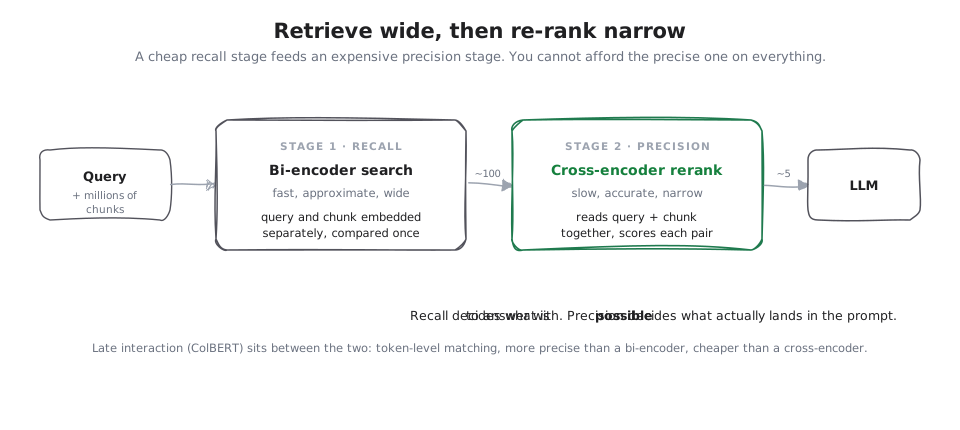
A re-ranker (usually a model called a cross-encoder) reads each candidate chunk together with the question, in one go, and scores how well the two actually fit. Reading them side by side is far more accurate than comparing two vectors that were made separately, because the model can see how the question and the chunk relate. It is also too slow to run over millions of documents, which is exactly why it only runs on the rough hundred the first search already found. The first search decides what is even in the running; the re-ranker decides what actually makes it into the prompt. Adding a re-ranker is often the single biggest improvement you can make to a mediocre RAG system.

Contextual retrieval: give the chunk its context back

A sentence torn out of a report, "the rate rose to 4 percent," is meaningless on its own. Which rate? Which year? Which company? Before you file that scrap away, you staple a note on top: "Acme, 2024, unemployment." Now it can be found for the right reasons.

When you split a document into chunks, each chunk loses the context of where it came from. A chunk that says "the rate rose to 4 percent" is useless if the retriever cannot tell which rate, which year, which company. Contextual retrieval, a technique popularized by Anthropic, prepends a short model-generated blurb to each chunk before embedding it, situating the chunk in its source document, and pairs contextual embeddings with contextual BM25. The chunk you index is no longer an orphaned fragment; it carries enough context to be found for the right reasons.

What to actually use

The honest default for most systems: hybrid retrieval (dense plus BM25, fused with RRF), a cross-encoder re-ranker as a second stage, and contextual retrieval if your chunks are losing their context. Reach for SPLADE or ColBERT when you need more retrieval quality than a bi-encoder gives but cannot afford to re-rank everything. None of these is exotic anymore, and stacking them is normal.

Getting the match right is half the battle. The other half is what you chose to index in the first place, which is the next piece.